An exploration of the different biological enrichment algorithms and machine learning algorithms applied to an RNA expression dataset.
Source Code: GitHub
Motivation
This project is an exploration of RNAseq data from Kaggle. When I initially downloaded this dataset, it was because I wanted to learn how to do data analysis on high dimensional biological data. Being a dataset with 370 x 50,000 features, I knew this would be a great way to challenge myself. Months later, I look back and realize I’ve come a long way. This project is a showcase of some the following skills applied to RNAseq
- Gene Set Enrichment Analysis (GSEA)
- Unsupervised Learning
- Variational Autoencoders — Latent Space Decomposition
Project Background
The dataset provides has 370 samples of patients. The samples for the RNAseq analysis were taken from four different regions of the brain: hippocampus, temporal cortex, parietal cortex, and white matter of the forebrain. Approximately 50,000 genes were identified across the 370 samples.
Gene Set Enrichment Analysis (GSEA)
GSEA is a technique made famous by Subramanian Et al (2005) in the paper Gene set enrichment analysis: a knowledge-based approach for interpreting genome-wide expression profiles. It aims at providing a framework for interpreting RNA expression data between two sample groups. It takes a genome library as an input, such as KEGG, and returns enrichment outputs to give biologists an idea of what metabolically relevant groups are unregulated in their systems. An example of a metabolically relevant group could include TCA Cycle, Lipid Metabolism, or Oxidative Phosphorylation genes.
From the RNAseq brain data, GSEA was run comparing two different sample areas of the brain: white matter of forebrain, and the hippocampus. The following is an example of one of the pathways that was identified as being enriched between the two groups.
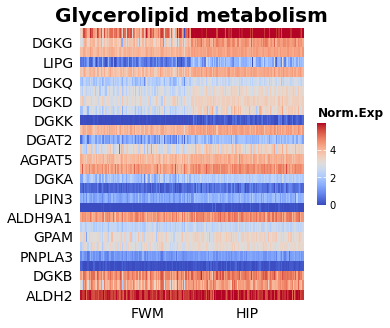
There is a visual separation between the two groups that is most evident at the top of the heat map. In this case, we had many patient samples, so this was one of the many pathways as enriched between the two pathways; enriched indicates that one sample has a higher expression of a pathway relative to the other group.
So from these patient samples, it looks like Glycerolipid metabolism has different activity across different pathways in the brain. Another useful way to visualize the enrichment between pathways is the enrichment score plot. This view is useful because we can see that a lot of our genes are randomly dispersed through our ranks, but there does seem to be a dense cluster on the right side for all these pathways. Understanding this is critical to make sure we’re not drawing too strong of conclusions.
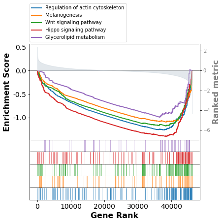
Since the RNA is coming from different areas of the brain, I don’t think it’s a surprise that there are different expression profiles between different biologically relevant groups. For this reason, I chose to investigate Gene Set Variability Analysis (GSVA).
Gene Set Variability Analysis (GSVA)
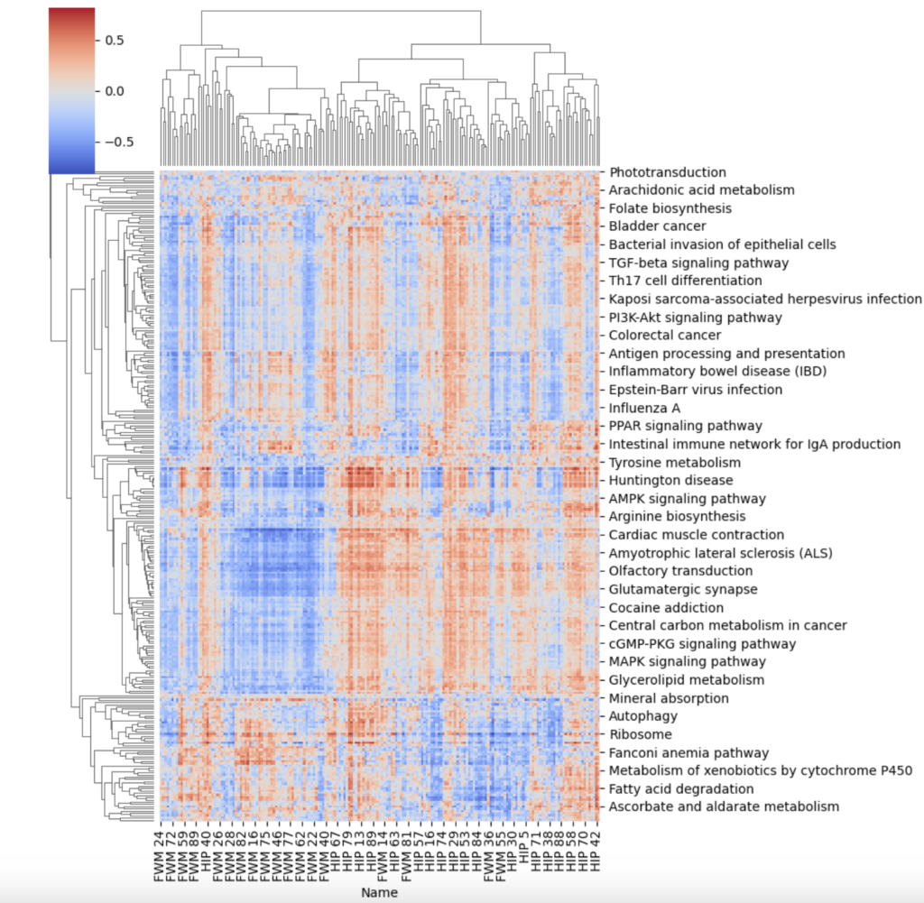
I chose to investigate gene set variability analysis since the GSEA method visually had a lot of heterogeneity despite finding enriched groups between the two sample conditions. Additionally, It was of interest to find sub groups within the patient RNAseq profiles. To do this, I created a cluster map of the GSVA results. Although still having a lot of heterogeneity, there are some sub groups within the population that be identified by the areas of intense blue or intense red, as well as the hierarchical cluster’s on the graph. If there was more metadata present for this gaining RNAseq dataset, it could be worthwhile to understand why some of the subgroups might be having different gene expression patterns.
Section 2: Modeling
Dimensional Reduction Algorithms
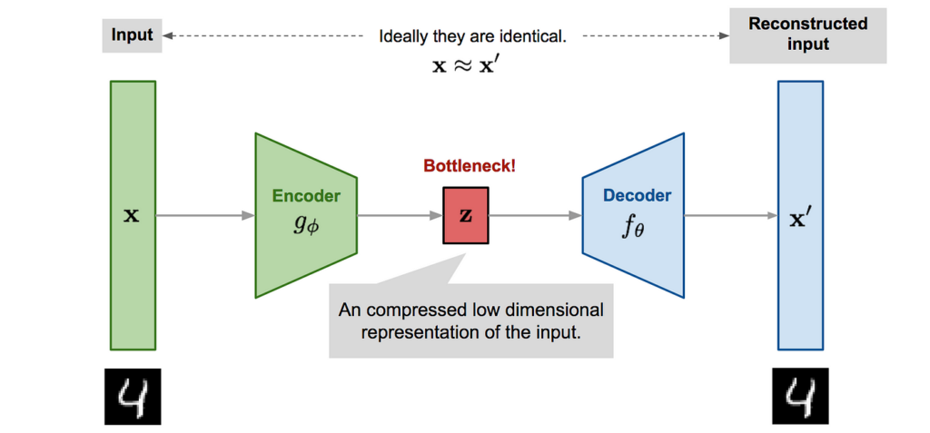
The Autoencoder is a type of neural network that introduces a bottleneck layer. This bottleneck layer can be used for latent space approximations of inputs. This type of latent space approximation can be thought of as a PCA latent space decomposition, but with one major difference — the latent space representation can be non linear with respect to the inputs. The introduction of nonlinear activation functions can introduce better latent space approximations, since many systems are nonlinear. The following is a diagram of what a autoencoder looks like.
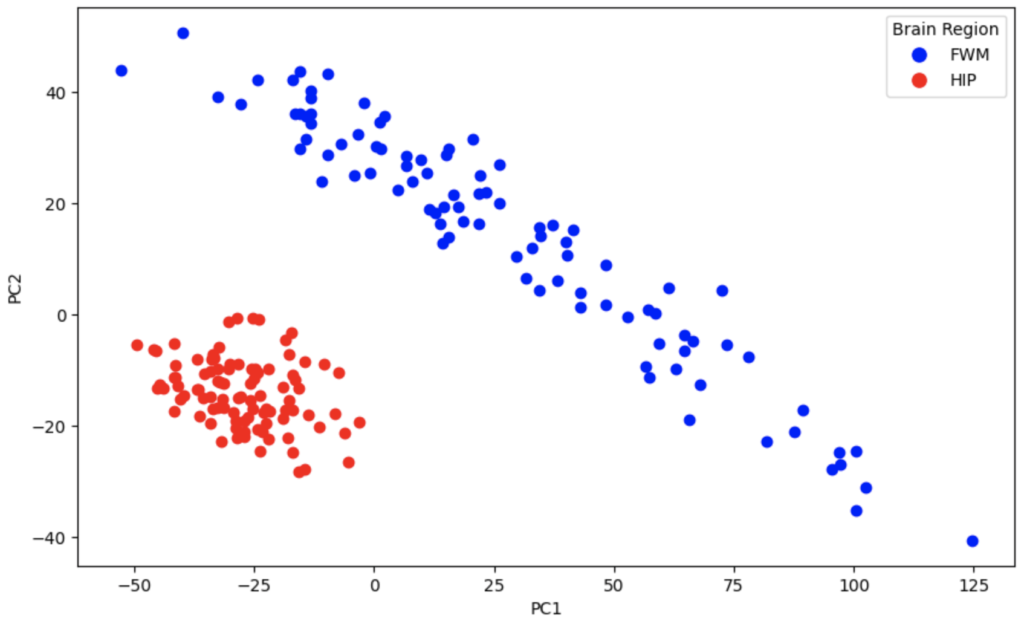
Before I show the outputs of the variational autoencoder, I’ll show the outputs of the PCA separation using n = 2 components. Explained variance with PC1 and PC2 is 32.6% and 9.4% respectively.
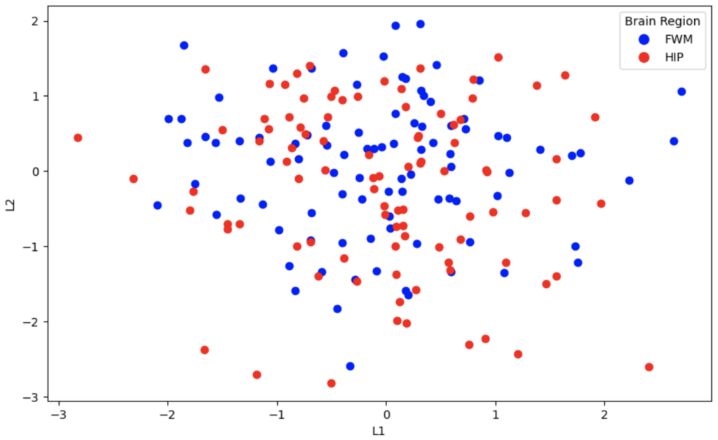
Now, we’ll show the latent space representations of the variational autoencoder.
Now I’ll show the outputs of the autoencoder. It’s interesting to see the nonlinear separation plane in 2D
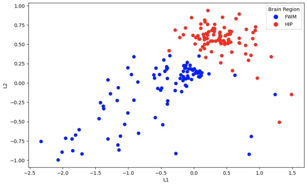
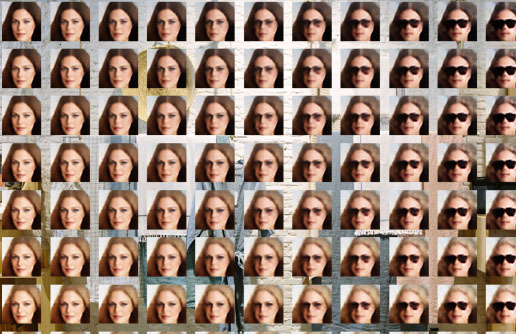
It’s evident that the PCA algorithm and autoencoder do a better job of separating these two classes in two dimensions. The reason that the VAE embeddings are so overlapped is that by definition, they produce a probabilistic distribution of embeddings for the original data. When the latent space is small, such as 2 outputs, the distributions overlap. When higher dimension latent spaces are used with VAE’s, they can be used to generate data that is similar to the original data by adding some noise. This concept is best understood when visualized for generative models of people’s faces; they are less suited for low dimension embeddings for training other models.
Naturally, my curiosity spiked wondering how these embeddings could be used to train another model. It’s worth mentioning that we know which area of the brain these samples were taken from, but one could imagine a similar situation where you performed RNAseq on patients and you are trying to perform some sort of classification i.e diagnosis/probability of a certain disease; the possibilities here are limitless and depend on the value they would bring. Out of curiosity, I looked into the following questions.
- How do these embeddings perform on a simple binary classification task
| Embedding Type | Accuracy Score |
| Variational Autoencoder | 50% |
| Autoencoder | 100% |
| PCA | 97.4% |
This is a very interesting finding since it presents a data scientist with the ability to produce highly informational nonlinear embeddings for training models or simply for visualizing high dimensional data in lower dimensions.
