Source Code: GitHub
Competition Overview
In this competition, you’ll develop machine learning (ML) models to predict the binding affinity of small molecules to specific protein targets – a critical step in drug development for the pharmaceutical industry that would pave the way for more accurate drug discovery. You’ll help predict which drug-like small molecules (chemicals) will bind to three possible protein targets.
To evaluate potential search methods in small molecule chemistry, the competition host Leash Biosciences physically tested some 133M small molecules for their ability to interact with one of three protein targets using DNA-encoded chemical library (DEL) technology.
Section 1: Final Approach
Project General Approach
This isn’t my first time experimenting with biological and drug-related data. I had a clearer picture in mind when approaching this problem due to courses/textbooks/research papers I’d studied and previous Kaggle Competitions. Using a Transformer Neural Network was without a doubt on my mind immediately. I knew that for a task like this, finding a meaningful feature space for the inputs. Along the way, I experimented with DeepChem molecule embeddings, ESM protein embeddings, one-hot encoding of amino acids, SGDClassifiers, XGBoost, Catboost, Random Forest, and neural networks. The largest challenges I faced along the way were vanishing gradients for neural network weights, memory constraints due to dataset sizes, computational overhead from I/O operations reading datasets, and time constraints to explore the hyperparameter space of models. Nonetheless, The following is the final refined workflow. Additional approaches are outlined in the proceeding section titled “Other Approaches”.
Computing Specifications
- AWS Sagemaker Notebook ml.g6.8xlarge instance for final workflow
- AWS S3 storage
- Dask, and Numpy arrays
Step 1: Drug Embedding
Previous to this competition, I’d encountered various fingerprinting methods found in the RDKit framework, but I wanted to try molecular graph decomposition using adjacency matricies. For this, I pursued two avenues: a self-created molecular decomposition embedding and embeddings through the DeepChem library.
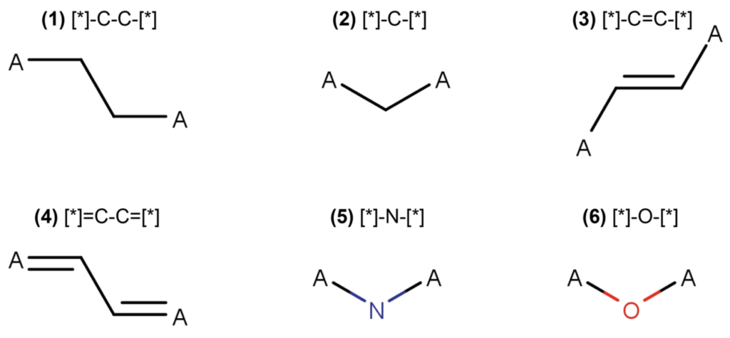
Using molecular graph decompositions seemed promising, but I was encountering issues with vanishing gradients in graph neural networks. I tried different learning rates and implementing different learning rate schedules, but I still couldn’t figure this out. I have a few hypotheses for possible remedies/sources for this issue.
- The nueral network architecture is too simple/complex
- A different weight initializing scheme is needed.
- More meaningful features need to be created
- A leaky ReLU is needed (one of the competition submissions used this)
Since this approach led to a bit of a dead end, I chose to go back to simpler embeddings that have successful use cases: MACCS keys and Morgan Fingerprints. Performing a quick analysis of the MACCS Keys and Morgan Fingerprints on a small subset (~300,000) of the data revealed the following. Note that cross-validation was not performed, but it’s a best practice to implement since covariate shift is a massive concern, especially with such a complex problem as drug binding. Precision, Recall, and F1 scores were used due to the class imbalance for drugs that bind and drugs that don’t bind.
| Embedding Type | Precision | Recall | F1 Score |
| MACCS Keys | 0.411 | 0.304 | 0.349 |
| Morgan Fingerprint (Radius = 2, n_bits = 1024) | 0.642 | 0.490 | 0.556 |
| Morgan Fingerprint (Radius = 2, n_bits = 2048) | 0.688 | 0.398 | 0.505 |
| Morgan Fingerprint (Radius = 3, n_bits = 2048) | 0.714 | 0.401 | 0.513 |
The evaluation metric for this competition was mean average precision, so I went with the highest precision embedding: Morgan fingerprints with radius = 3 and n_bits = 2048.
Data Subset
5.5 million data points were randomly taken from the 300 million row subset using the parquet files and a library named duckdb. The smiles were taken from each of the rows of the subset dataset and converted to Morgan fingerprints; the final data dimensions were 5.5 million x 2048. Below is a snippet of what the original train dataset looks like, excluding the column that dictates whether a molecule binds to a given protein.

Step 2: Protein Embedding
At their very foundation, proteins can be characterized by their primary, secondary, tertiary, and quaternary structures. The primary structure is the full amino acid sequence that defines these proteins. These sequences are readily available on uniprot.org. Secondary and tertiary structures can be either determined experimentally or predicted with AlphaFold2. Quaternary structures can also be predicted using AlphaFold2. From these four levels of structure, the following types of embeddings can be performed
- One Hot Encoding of Amino Acid Sequences
- Hidden Layer embeddings with Nueral Networks
- Spatial Embeddings using protein contact maps
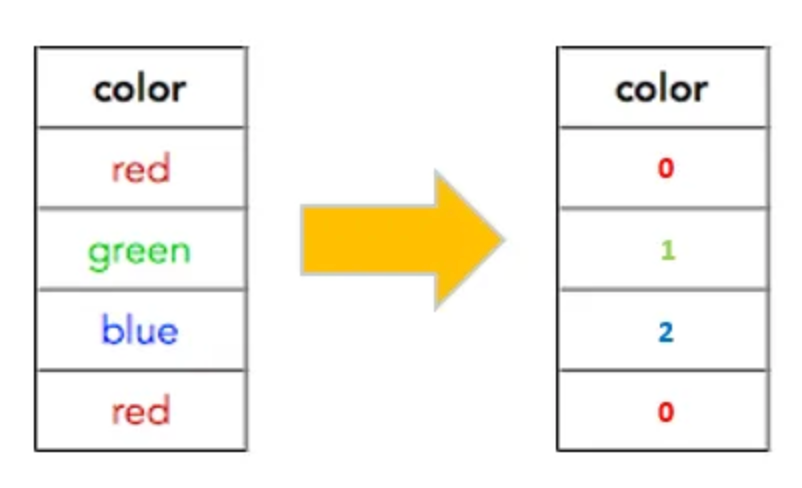
Depending on which embedding you choose, there are varying levels of computational power that will be needed in terms of memory, GPU, and any I/O operations for saved variables. Due to the tremendous amount of computational overhead that I couldn’t sustain with a ml.g6.8xlarge instance, I chose to perform a simpler label encoding of each protein. The following is an example of label encoding.
Step 3: Model Building
So the model choice and hyperparameters for a model can be important, but from my experience, having rich input features for a model is the most important part, aside from situations where a transformer neural network has proven applications. That being said, the model choice and hyperparameters can be important to make sure that the model is not overfitting. The following were models that were evaluated during the duration of this competition.
- XGBoost Classifier
- CatBoost Classifier
- Fully Connected Nueral Networks
- Graph Nueral Networks
- Stochastic Gradient Descent Classifier
The final model that was used for the model submission was an XGBoost Classifier; this provided the best score for the Kaggle leaderboard. The XGBoost model is a gradient-boosting model with lots of hyperparameters, but only a subset of these were explored: subsample, n_estimators, max_depth, and subsample. In the end, the cost of exploring these hyperparameters was taking a very long time, and the cost associated with the AWS instance was too much for my budget. So, I chose to use the base parameters of the model.

The other models explored produced similar test results or worse, but again, the hyper-parameters were not properly explored.
Final Competition Outcome
At final competition evaluation, the hosts of the competition reevaluated everyone’s model based on a hold-out test set that was not included in the submission scores; the test data was released to everyone, but leaderboard rankings were for only 35% of the test dataset. My final placement in the competition was 1428/1948 was mean average precision score of 0.133. While I wish I would’ve done better, it’s worth noting that the winner of the competition only had a mean average precision of 0.306. As a whole, the task of predicting small molecule binding to proteins is in its infancy.
With more computation power, I’m confident that I would’ve been able to increase my rank.
Section 2: Alternative Approaches
A. Embeddings:
Primary Structure
The primary structure of a protein is rich in information, typically containing hundreds of amino acids. Thankfully, the computational biology community has created models that can take these primary structures and convert them into feature-rich numerical embeddings for machine learning. One model that can do this is ProtBert by Rostlab. This model was leveraged for embeddings in this project.
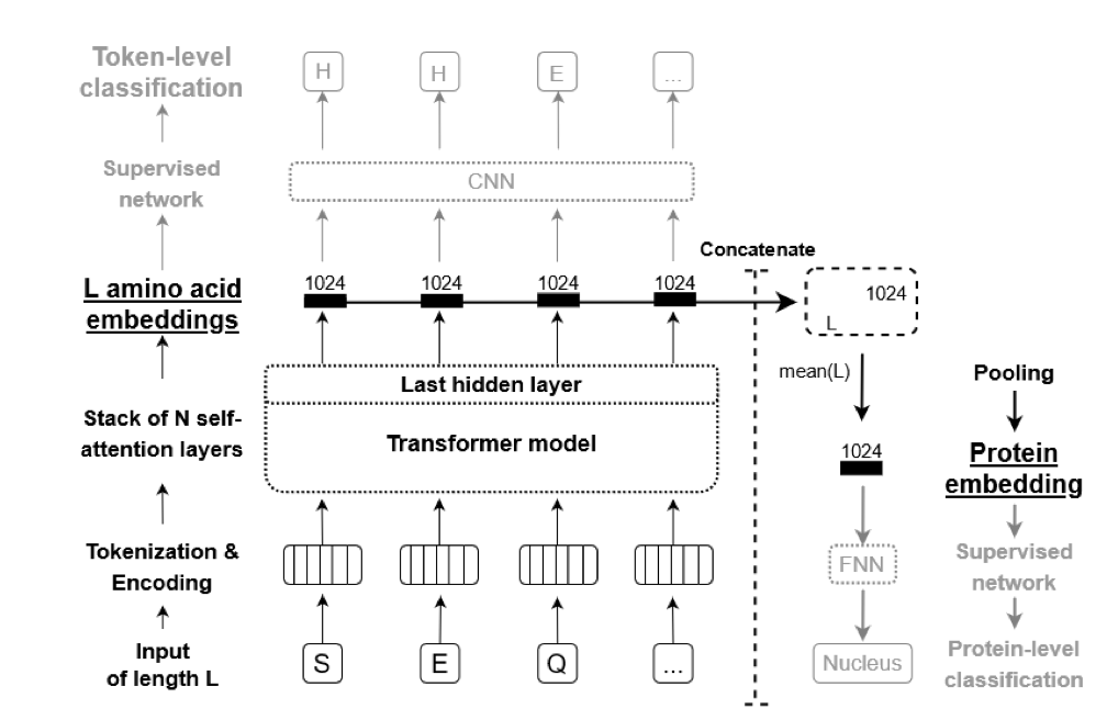
These amino acid embeddings served as the input to a neural network that was attempted. The training of the neural network ended up being difficult; the training loss stalled after one epoch. I did notice with the final competition submission that someone used a LeakyRelu for their activation functions, whereas I used a Relu activation function. This is something to consider/attempt in any future neural network models where the training loss is stalling.
Secondary Structure and Tertiary Structure
To pursue embeddings involving secondary and tertiary structure, one could search up the experimental structure or download the computational structure from AlphaFold2. The following is an example of what the predictions coming out of alpha fold might look like

Wow isn’t that beautiful! Unfortunately, this alone is not enough to embed the information into a machine-learning model. A protein contact map needs to be generated. Inevitably, there are some hyperparameters for generating these contact maps. I have not attempted this form of embedding and assessed its performance but, the result would look something like the following.
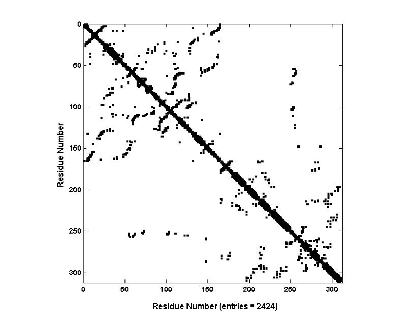
The steps for generating these contact maps can seen below.
Steps to Generate a Protein Contact Map
- Obtain the 3D Coordinates:
- You need a structure file (e.g., PDB format) with the 3D coordinates of each atom in the protein. This can come from a database like the Protein Data Bank (PDB) or a structure prediction tool like AlphaFold.
- Choose a Distance Threshold:
- Common thresholds range from 5 to 8 angstroms, representing whether two residues are considered in contact.
- Calculate the Distances:
- Calculate the distances between the atoms of all pairs of residues. This is usually done by considering the distances between the C-alpha atoms or any representative atoms for each residue.
- Define the Contact Map:
- Create a 2D matrix with a dimension matching the number of residues.
- If the distance between two residues is within the threshold, mark the corresponding cell as “1” (contact) or “True”; otherwise, mark it as “0” (no contact) or “False”.
B. Model Alternatives
Up to this point, the protein amino acid information has been embedded into its own set of features, and the chemical structures of our pharmaceutical drug candidates have been incorporated into graph decompositions that can be fed into graph neural networks. Given we have two separate inputs, it makes sense to have two separate parallel networks that eventually concatenate, as seen below.
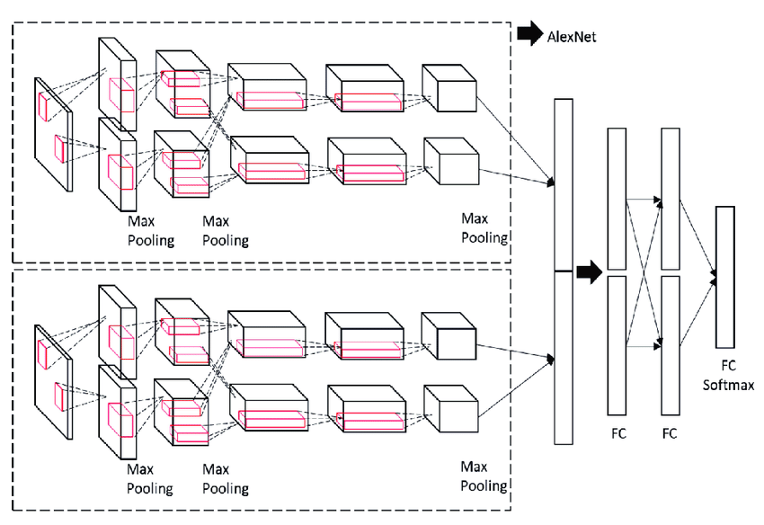
The above image shows two parallel convolutional models being concatenated into a fully connected layer. For this model, a fully connected layer could be used, or additional transformers could be applied to the concatenated layer to learn more features.
At this point, I didn’t know which would perform best. Transformers can learn complex feature relationships, but some of the inputs have already been created using transformers, so would this be necessary? Putting a fully connected layer on top of the two parallel models was simpler and would probably be more computationally efficient. I was certain this would be something I would investigate during this competition.
Simple GCN with Fully Connected Layer Deep Learning
I chose to investigate deep learning for this model, as opposed to other methods such as gradient boosting, because PyTorch has very developed Modules that support incorporating node and edge features along with the original adjacency matrices that represent connections. The following is a snippet of code for the first model structure investigated.
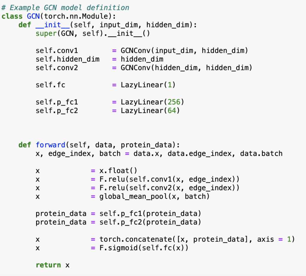
The purpose of creating this simple model was to gauge how rich the features were being input into these neural networks. The preliminary experiment involved loading subsets of the training data. One million data points from the training set were loaded, and after some preliminary exploratory data analysis, it was obvious that there was a very extreme class balance. I chose to incorporate all the data points that involved a drug binding to a protein target, and around 10-20 thousand samples of drug-protein combinations that didn’t show binding.
As mentioned in Section 1, I had issues with the learning stalling after epoch 1. I tried adjusting the learning rate scheduler and learning rate, but I kept running into the same problem. Seemingly, I ran into a case where the prediction task was difficult, and learning the function that describes the situation in the neural network was difficult. As mentioned, I saw a solution that used LeakyRelu as the activation function and this worked well. I think the model that I created might have been too simple as well. It probably would’ve been worth it to use multiple blocks of the same structure, such as a transformer. That being said, I was already running into issues with computation so increasing complexity was not going to help!
Conclusion
I would love to explore this neural network route more in the future with the proper resources. Ultimately, it was a good introduction to graph neural networks and the difficulties that come with neural networks.
