Nextflow is a powerful workflow management tool designed to streamline and automate data processing pipelines, particularly in bioinformatics. By leveraging domain-specific language (DSL) syntax, Nextflow enables researchers to write complex workflows that are portable, reproducible, and scalable across various computing environments, including local workstations, high-performance computing clusters, and cloud platforms like AWS. Its ability to manage dependencies, parallelize tasks, and efficiently handle large datasets makes it particularly valuable in RNA sequencing (RNAseq) workflows, where it can orchestrate the alignment, quantification, and differential expression analysis steps. With support for containerization through Docker or Singularity, Nextflow ensures consistent environments across different stages of the workflow, significantly enhancing reproducibility and minimizing issues related to software versioning. This robust framework is thus instrumental in advancing reproducible research in data-intensive fields.
The following writeup will go over the practical implementations of a NextFlow RNAseq pipeline from the nf-core community, more specifically Patel et al., 10.5281/zenodo.1400710.
I. Background and Methods
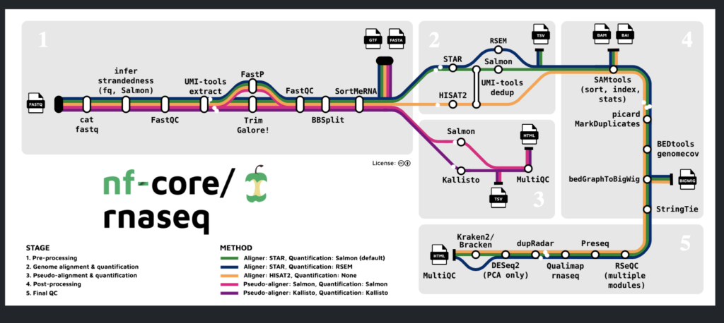
The pipeline seen above is the RNAseq pipeline created by the nf-core community. It offers a series of quantification, quality, and visualization tools that together provide a gold standard for analysis. To use the NextFlow pipeline above, each of these tools needs to be installed and properly setup, along with a containerized service such as Docker or Singularity. Using a Linux environment is preferred since many of these tools have linux-based binaries. Depending on the Linux operating software, sudo yum or sudo apt-get can be used to install many of these softwares, while some of these softwares are more easily installed using the python installation (pip) manager or R’s installation manager.
After installing all necessary software, the next step is to create a sample sheet for the samples intended for the pipeline. To set up the workflow, an E. coli sample was used initially to test the pipeline before moving on to more computationally intensive samples, such as those from human tissue. This test sample (SRR959239) was downloaded from NCBI’s Sequence Read Archive

Once the sample sheet is setup, the following additional parameters need to be specified.
- outdir: The output directory for the processed files that come out of the nf-core pipeline
- gtf: The genome annotation file used for identifying genes in a given genome
- fasta: The genomic sequence for a given genome
- profile: The container service to be used
NextFlow nf-core requires that sample sheets be setup in the format seen in Figure 2. Below is an example of a sample sheet for a single sample; if multiple samples are used, the format remains the same, with each sample added as a new line.


If everything has been set up correctly, the Nextflow pipeline will start running in the terminal, displaying the status of various processes throughout its execution. Once the pipeline completes, several folders will be generated in the output directory, including fastqc, multiqc, pipeline_info, star_salmon, and trim_galore. The multiqc folder contains the multiqc_report.html, which provides the most comprehensive summary of the pipeline’s run status. We’ll slowly go through the major elements of the quality control report. Note that MultiQC was designed to provide an easy to use Graphic User Interface (GUI) for multiple samples, but only one true sample is shown below
MultiQC Outputs
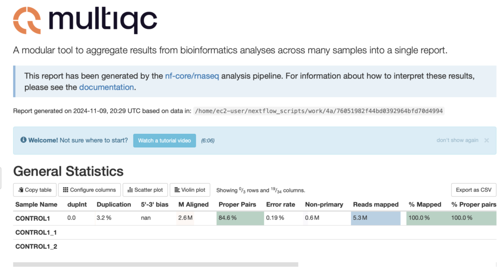
The General Statistics section in a MultiQC report provides an overview of key metrics and summary statistics for multiple samples or datasets within a single report. It consolidates results from various bioinformatics tools into a unified table, allowing for easy comparison across samples. This section is essential for quickly assessing data quality and identifying any anomalies or outliers across samples in the analysis pipeline, aiding in making informed decisions on further steps. The general statistics for this sample appears to have no reg flags.
FastQC
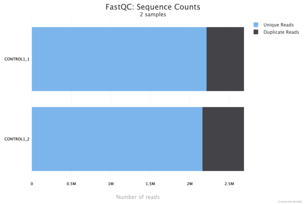
The Sequence Counts plot from FastQC in a MultiQC report displays the total number of reads in each sample, offering an immediate visual summary of sequencing depth across the dataset. This plot helps identify any significant discrepancies in read counts between samples, which can indicate issues like sequencing failure, sample loss, or other technical variations. Consistency in sequence counts is often desired for balanced downstream analysis, so this plot is useful for detecting outliers or samples that may require additional attention, such as re-sequencing or further quality control. The two fastq inputs appear to be well balanced, indicating re-sequencing or further quality control is likely not needed.
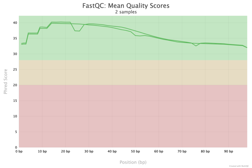
The Quality Score plot from FastQC in a MultiQC report provides a comprehensive overview of the per-base quality scores across all reads within each sample. This plot is crucial for assessing the reliability of sequencing data, as it visualizes how quality scores fluctuate along the length of the reads. Typically, higher scores at the start of reads indicate good sequencing quality, while scores may decrease toward the end of reads due to sequencing limitations. Samples with consistently high scores are preferable for downstream analyses, as poor quality can affect alignment and variant calling accuracy. The plot also helps identify any samples with significantly lower quality, which may need to be trimmed or filtered before further processing. This visual summary supports quality control efforts by allowing researchers to make informed decisions about the usability and processing of each sample.
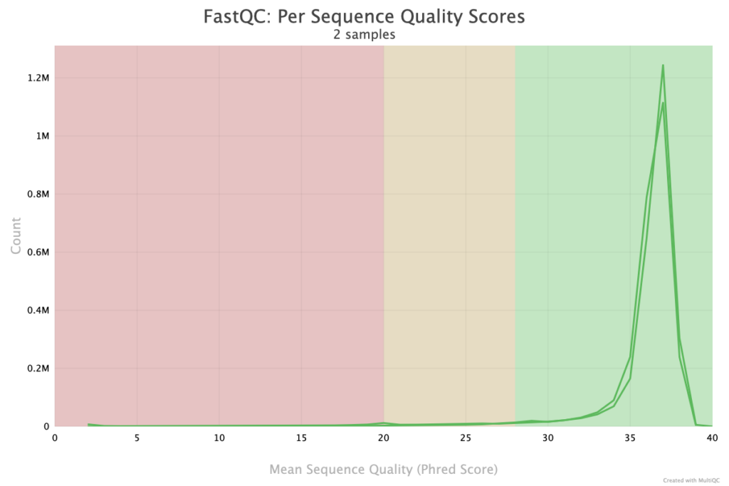
The Per Sequence Quality Scores plot in MultiQC provides insight into the average quality scores of individual reads within each sample. This plot is essential for evaluating the overall quality distribution across all reads, helping identify samples with consistent high quality as well as those with potential issues. Ideally, the plot should show a peak at the high-quality end, indicating most reads are reliable. A spread or secondary peak at lower quality scores might suggest potential problems, such as degraded samples or technical issues during sequencing. This view enables researchers to detect samples with substantial proportions of low-quality reads, which may need quality filtering or adjustments before proceeding with downstream analysis. By summarizing read-level quality, this plot aids in early identification of problematic samples that could otherwise introduce noise or errors in the analysis.
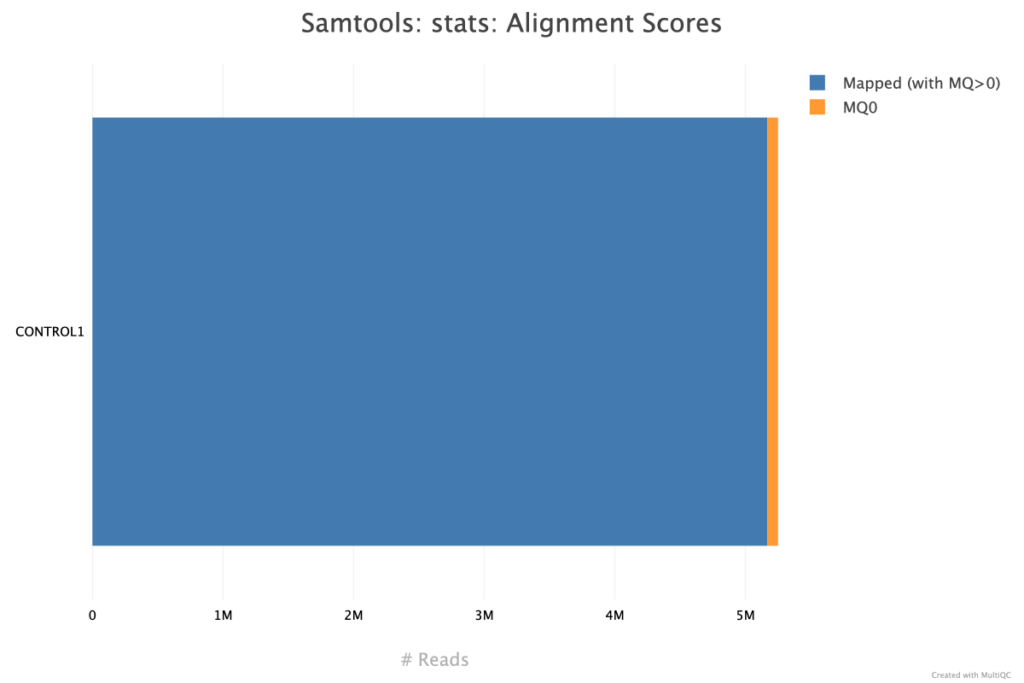
The alignment scores provided by Samtools in a MultiQC report give a summary of read mapping quality across samples, often including metrics like the percentage of aligned reads, unmapped reads, and the proportion of properly paired reads. High alignment percentages typically suggest good sample quality and compatibility with the reference genome, while lower percentages may indicate sample contamination, poor-quality sequences, or an inadequate reference genome. Properly paired reads are also critical in paired-end sequencing, as they ensure correct fragment size and alignment orientation, adding reliability to downstream analysis. These Samtools alignment metrics are valuable for evaluating the effectiveness of the alignment process and identifying any potential issues with sample quality or compatibility. The Samtools alignment scores for these fastq files does not have any major issues
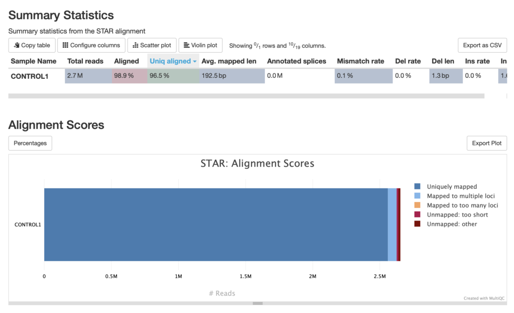
The alignment scores generated by STAR (Spliced Transcripts Alignment to a Reference) and visualized in MultiQC focus on RNA-seq data, where accurate alignment across exon-exon junctions is crucial. STAR provides a range of alignment metrics, including the percentage of uniquely mapped reads, multi-mapped reads (those aligning to multiple locations), and unmapped reads. High percentages of uniquely mapped reads indicate high-quality RNA-seq data, while multi-mapped or unmapped reads may suggest repetitive regions, contamination, or low-quality sequences. STAR’s ability to align reads spanning splice junctions makes it particularly valuable in transcriptome studies. The data ran for this analysis appears to be very high quality.
Conclusion
To access the results from the gene alignment, navigate to the star_salmon folder within the output directory that was specified. Within that folder, a list of files and folders similar to those below will be seen.
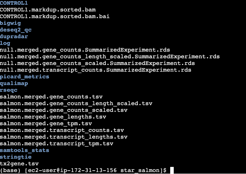
As can been seen, a ton of data is generated for a single alignment. Thankfully much of the critical data is summarized in the multiqc report shown earlier. From the image above, the salmon gene counts can be seen with various preprocessing techniques applied to them.
As an analyst that likes to control the destiny of the data, starting with the salmon.merged.gene_counts.tsv file would be preferred. This file contains the raw gene counts as determined by Salmon. Note that Salmon doesn’t strictly count reads in the way that aligners like FeatureCounts do. Instead, it uses quasi-mapping or alignment-free approaches to estimate the likelihood that a read originated from each possible transcript or gene. When a read maps ambiguously to multiple transcripts or genes, Salmon assigns a probability to each possible source. As a result, the gene counts file will have some genes with non-integer gene counts.
Next Steps
At this point, the raw gene counts are ready for downstream analysis. The downstream analysis of the count data generated is outside the scope of this analysis. Downstream analysis of count data can be found in this portfolio.

