Background
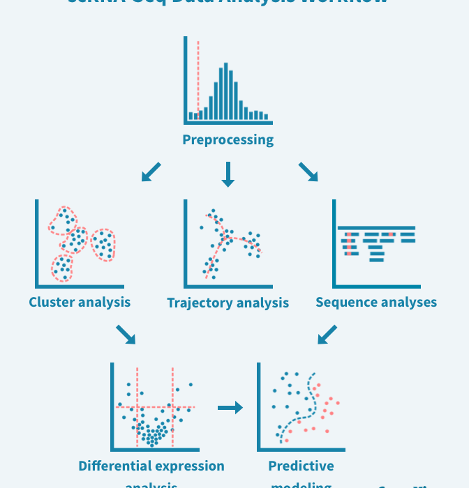
Single-cell RNA sequencing (scRNA-seq) is a cutting-edge technology that enables the analysis of gene expression at the level of individual cells. This method allows researchers to explore the heterogeneity within a population of cells, identifying distinct cell types, states, and responses that would be masked in bulk RNA sequencing. By isolating and sequencing RNA from thousands to millions of single cells, scRNA-seq provides a detailed map of cellular functions, developmental pathways, and disease mechanisms. It has revolutionized fields like developmental biology, cancer research, and immunology by uncovering rare cell populations and revealing how cells interact and evolve in complex biological systems. This technology has become an essential tool for understanding cellular diversity and dynamics across various tissues and conditions.
In this workflow, Ulcerative Colitis patients were subjected to sc-RNAseq. Additional healthy controls were included. The main study design is summarized below
- 30 Subjects
- Patient Health (Disease, Healthy)
- Location of Colitis in Colon (Origin)
- Gender (Male, Female)
- Smoker History (Current, Previous, Never)
Additional metadata provided in the original annotated data (AnnData) can be seen below.
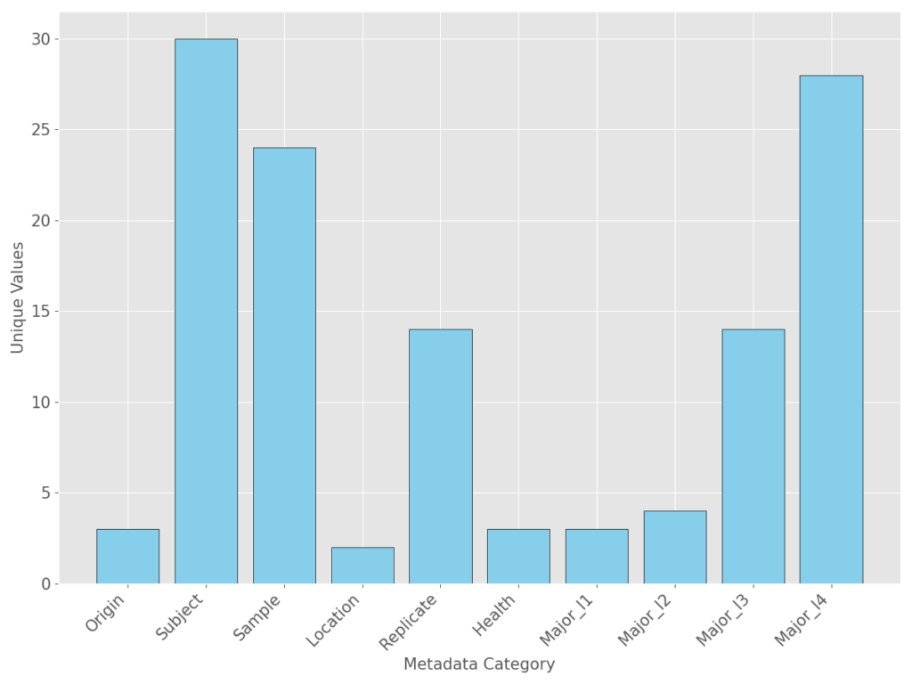
- Origin — location that the sample was taken from (laminar propria, epithelium, fibroblast tissue)
- Subject — Unique identifier assigned to each patient/healthy control in the study
- Sample — Sample identifier associated with the replicate and location id of the sample. Most samples had two epithelial samples and two laminar propria samples. This metadata is a combination of the location and replicate fields
- Location — Additional metadata indicating if the sample was laminar proprial or epithelial
- Replicate — Additional metadata containing the replicate information
- Health — Status of the tissue/patient sample (Non-inflamed, Inflamed, and Healthy)
- Major l1-l4 — Cell annotation information that was not used
This dataset was made publicly available and provided by Smillie el al., 2019 through Pertpy. The cell annotation information in the original dataset was ignored. The final annotations are compared to the original annotations in the dataset in the final section of this workflow. The Pertpy scRNAseq dataset summary can be seen below.
| UMI Sequenced | 365492 |
| Total Genes Captured | 18172 |
I. Background and Methods
Single Cell RNAseq data provides extreme detail and granularity that were not possible before, but comes with associated risks that must be handled in the preprocessing workflow. Due to the AnnData object provided by Scanpy, many different transformations of the single-cell data can be saved allow preprocessing with different algorithms to deal with weaknesses such as low quality cell removal, doublet identification, ambient RNA removal, and feature selection.
In single-cell RNA sequencing (scRNA-seq), removing low-quality cells is a critical preprocessing step that improves data reliability and biological interpretation. One common indicator of cell quality is the proportion of mitochondrial RNA; cells with high mitochondrial RNA levels often indicate cellular stress or damage, as they may release more mitochondrial transcripts due to compromised membranes. Cells with excessive mitochondrial gene expression—typically above a defined threshold—are flagged for removal. Other metrics, such as low total gene counts, which may indicate dying cells or cell debris, and unusually high gene counts, potentially pointing to cell doublets or multiplets, are also used to filter low-quality cells. Ambient RNA may also be present from dead or damaged cells. These quality control measures ensure that downstream analyses focus on viable, biologically representative cells, leading to more accurate insights into cell-type-specific gene expression.
Mitochondrial RNA Removal
As mentioned above, excessive mitochondrial gene expression can be indicator of leaky mitochondrial membranes, indicating dead cells. As always, one must be careful when assigning thresholds. The underlying biology should always dictate abnormality. For example, brain cells tend to have higher mitochondrial cells as oppose to a less active cell type such as skin cells.
Annotating mitochondrial cells can be achieved using a range of manually curated libraries. A widely used resource for cell annotations is the Ma’ayan Lab’s Enrichr libraries. In this workflow, the Gene Ontology Cellular Component 2023 library was selected, as it categorizes genes based on their subcellular locations. For mitochondrial genes, this includes detailed subsets that specify whether the genes or their protein products are located in the mitochondrial matrix, inner membrane, or outer membrane. To ensure comprehensive coverage of all mitochondrial components, the following code snippet was used to identify and annotate any gene associated with components containing “mitochondria” in the name.
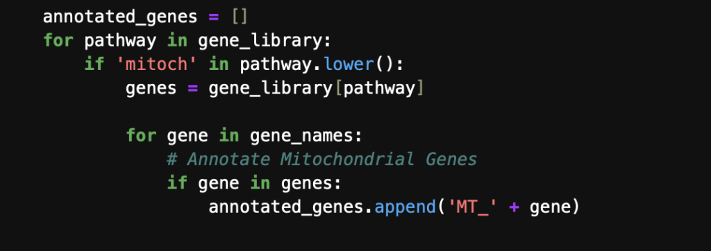
Following the annotation of cells, thresholds were set for the percentage of mitochondrial gene expression based off of two metrics: percentage of total mitochondrial genes and median absolute deviations of mitochondrial gene expression. The percentage of total mitochondrial genes is user set threshold that is determined on a case-by-case basis — set to 20% for colon cells. The median absolute deviations (MAD) is a measure of spread of the data that can be more robust than standard deviation for non-normal distributions. Gene expression data is known to follow a non-normal distribution and is often modeled by a negative binomial distribution, which is similar to a Poisson distribution, differing mainly in the assumption that the mean is equal to the variance. The negative binomial distribution allows for the variance to be a function of the mean, which holds true for gene expression data since the gene expression becomes more variable at higher abundances. The MAD set in this workflow can be found in the source code. Some of the plots used for sanity checks and decision of reasonable thresholds can be seen below.
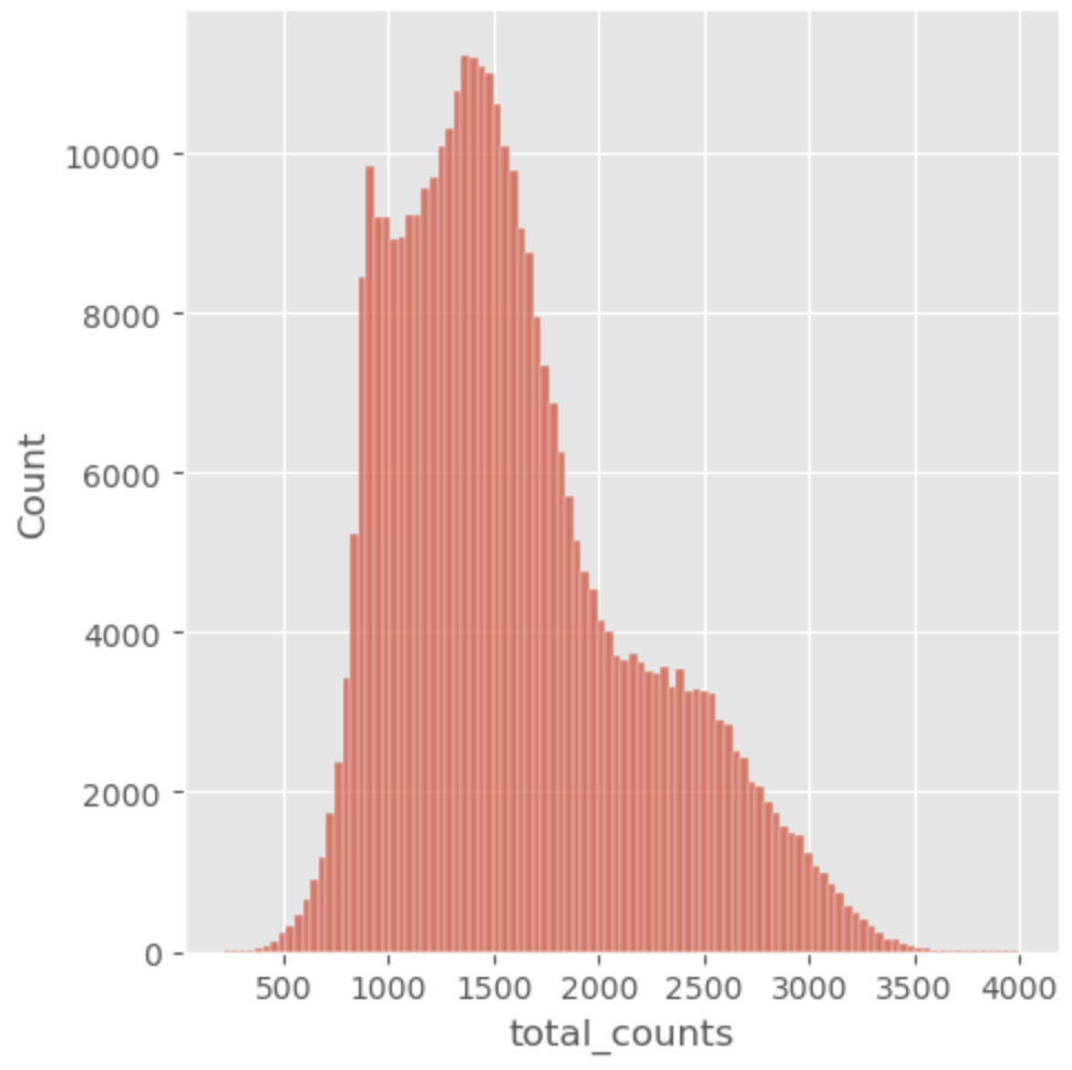
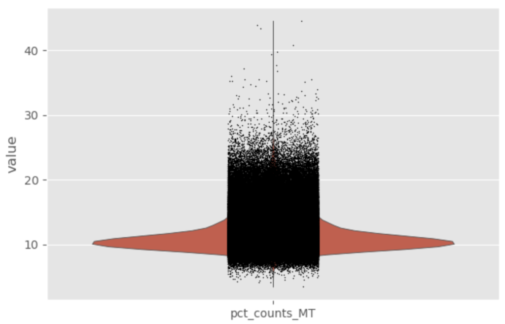
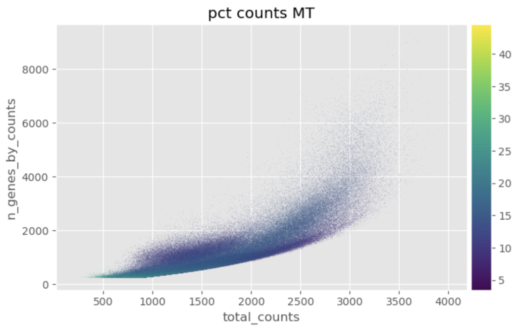
Once the cells were filtered for the percentage gene expression thresholds and MAD, further preprocessing was performed.
Doublet Identification
Doublets are a result of the technology used for sequencing cells. 10X genomics has a droplet based technology that tags cells uniquely one-by-one through a small capillary, as illustrated below.
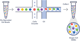
In an ideal scenario, each cell is encapsulated in the oil above individually and the corresponding UMI with gene counts is truly representative of a single-cell. However, in real world scenarios, it is expected that some portion of the cells encapsulated in the oil droplets, while two or more cells, which can heavily influence the analysis if not dealt with; the amount of loading material in the preprocessing workflow can increase the chances of this occurring.
To handle this phenomena, doublet identification algorithms have been created. Most of these algorithms developed are in the R programming language. The package used in this workflow for doublet detection was the scDblFinder, which is a part of the Bioconductor family of packages. Notably, this algorithm only detects heterotypic cells, which are cells that contain two separate cell types.
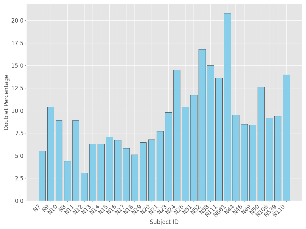
Since these samples were not processed in house, a critical decision had to be made on whether to perform doublet detection on all subjects vs one subject. Biopsies were performed at separate times, in different environments, with hopefully identical sample handling procedures. That being said, with any high throughput technology comes extreme sensitivity from the equipment and operator. With prior experience of other high throughput technologies, the logical approach ultimately indicated processing each subject individually for doublet detection. The following is a summary of the doublets identified for each subject.
Ambient RNA removal
Ambient RNA, or background RNA contamination, arises in single-cell RNA sequencing when RNA molecules from lysed or damaged cells remain in the suspension medium and get captured alongside intact cells. This can happen during sample preparation steps, such as dissociation or cell sorting, where some cells may break apart, releasing their RNA into the surrounding fluid. In platforms that encapsulate cells into droplets, such as 10x Genomics, these free RNA molecules can enter droplets and adhere to or mix with RNA from other cells, leading to contamination. Ambient RNA can skew expression profiles, especially for highly expressed genes, and impact the biological interpretation of single-cell data, making it essential to account for in analysis. To handle the ambient RNA, SoupX was used also in a batch-wise manner on a latent representation of the data created using PCA, UMAP, and leiden clusterings in that order; the leiden clusterings were the final latent representation of the data. The leiden clusterings were used because ambient RNA has been shown to be captured as a batch effect.
INSERT AMBIENT RNA CORRECTION PLOT
Feature Selection
For feature selection, there are several methods available. In Scanpy, the highly_variable_genes function can be used, implementing either the Seurat or Cell Ranger approach based on dispersion. This function requires log-transformed counts as input. However, it has been argued that using log-transformed counts can introduce bias, particularly in low-count genes. For example, adding one count to a gene with only two transcripts significantly increases its apparent variability.
To address this, an alternative method using raw counts—called deviance—was applied. Deviance-based feature selection models gene counts with a negative binomial distribution. Genes that deviate from this distribution are identified as highly variable, as they differ significantly from what would be expected under a standard negative binomial model. The deviance, a statistical measure, is calculated to quantify this difference, and the top 4,000 most deviant genes are selected for downstream analysis.
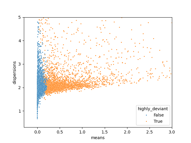
Importantly, the negative binomial distribution tends to be left-skewed, which aligns well with the characteristics of RNA sequencing data.
At this point, the data preprocessing has been adequately performed and ready for downstream analysis of the single-cell data. the A special thanks to the Theis Lab and all its collaborators for offering guidance in this analysis through online publications.
II. Cell Annotations
Now that the 4000 most deviant genes have been chosen, downstream analysis can be performed to annotate the cells in our experiment. For annotation, it’s useful to look at the UMAP representations of our data. Below are a couple UMAP representations that are extremely useful when considering cell type annotations.

The location of the epithelium samples are all mostly clustered together on the UMAP. This is a critical piece of information, since we should not see a high proportion of cell types that haven’t been in epithelial tissue. This figure will be referred to when making a final decision on whether the cell types annotated are accurate. Note that the following workflow will do manual annotations. Automated annotations have been proposed and shown to work, but they do heavily depend on the data used to train them and the data they are applied on. As usual, the concept of covariate shift applies to the data analysis here, so any automated annotation should be performed with caution. For this reason, the manual annotation format was performed. The first step in the manual annotation, was to perform leiden clustering using a resolution of 0.15 in scanpy.
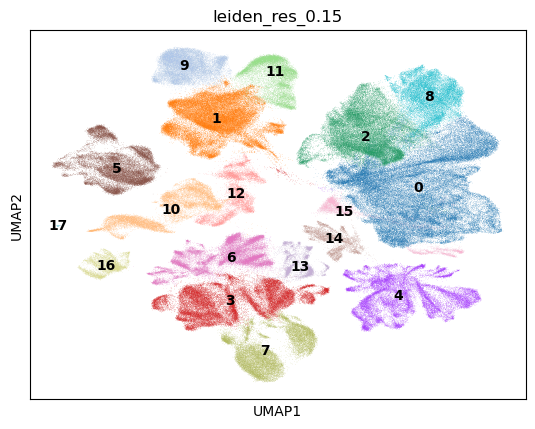
Each of the clusters in this image is supposed to represent a biological cell type. The hyper parameter in this scenario is the resolution, which as increased, gives more cell types. Since this was a first run through on cell types for this data, it made more sense to get larger cell type groups first and work down from there. As a result, the next step involved getting marker cells. During this process, the following websites were explored for possible markers.
- CellMarker (http://xteam.xbio.top/CellMarker/) — Does not contain digestive tract cells
- PanglaoDB (https://panglaodb.se/) — Contains GI Tract Cells
- Human Protein Atlas (https://www.proteinatlas.org/) — Contains Glial and Endocrine Cells
- Tabula Sapiens (https://www.ebi.ac.uk/gxa/sc/experiments/E-CURD-88/results/marker-genes) — Marker genes and clustering available on website
- Single Cell Expression Atlas (https://www.ebi.ac.uk/gxa/sc/home)
- Gastrointestinal Cell Atlas
Interestingly, the markers pulled from these websites were alright, but nowhere near the quality of the markers provided by ChatGPT4 o-preview. ChatGPT4 o-preview suggested the following.
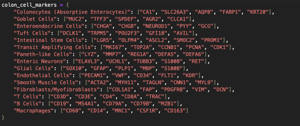
From the markers provided, the following series of plots were created to see if the markers provided highlighted regions identified by the Leiden clustering on the UMAP. Note that the following images are in sequential order of the colon cell markers dictionary in Figure XX i.e. Colonocytes, Goblet Cells, and Enteroendocrine Cells are the first four markers.
From the markers in the slides above, and the leiden clusterings, the following annotations were added to the UMAPs.
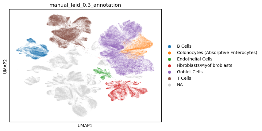
At this point, further annotations could be pursued to fill in the rest of the map and add more granularity to the cell types i.e. subsets of B cells.
Transfer Learning Annotations
Cell type annotation in single-cell RNA sequencing (scRNA-seq) has advanced with variational autoencoder (VAE)-based frameworks like scArches, which enable efficient transfer learning and model adaptation. By using VAEs, scArches learns a compressed representation of complex scRNA-seq data, facilitating the alignment of new datasets with existing, well-annotated reference datasets, such as the comprehensive gut cell atlas. This process allows researchers to map cell types in new datasets by leveraging learned patterns from the reference, reducing the need for manual annotation. VAE-based models in scArches are particularly valuable in distinguishing subtle cell types, as they can harmonize data across different experimental conditions and reduce batch effects, which is essential for consistent and accurate cell type identification in complex tissues.
To use a variational based autoencoder for label transferring, one must first obtain a reference dataset. In this workflow, colon cell atlas reference dataset was used. Once a reference dataset is obtained that has cell types annotated, the dataset must be used to train a variational autoencoder. The variational autoencoder used in this workflow was the SCVI autoencoder from scArches, mainly because scArches offers a seamless workflow for using AnnData objects directly. Without a doubt, one could design their own variational autoencoder and get similar results. Since I have experience using the software tools derived from the Theis Lab, I trust that their implementation is good. After training the variational autoencoder on a reference dataset, we must ensure that the dataset we are using has the same features. In other words, we make sure that the genes we trained the VAE with are present in our query dataset, or we handle the missing genes in some way. It made sense to check which genes were present in the query dataset from the colon cell atlas dataset before training the VAE, so this was done; approximately 3400 of the 4000 genes that were identified as highly deviant earlier in this workflow were in the reference dataset.
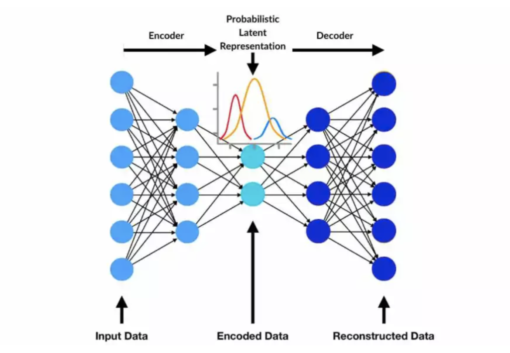
After training the variational autoencoder (VAE), the query dataset can be processed through the model to generate latent representations of the cell types. These latent representations can then be visualized to better understand the distribution and relationships among cell types.
It’s important to note that all subsequent figures are sourced from the single-cell best practices guide. This is due to challenges encountered in the AWS SageMaker JupyterLab environment, including memory limitations during neighborhood clustering of latent space representations and unresolved software dependency issues with Conda. Despite these obstacles, the following example demonstrates what such a visualization might look like for a query and reference dataset.
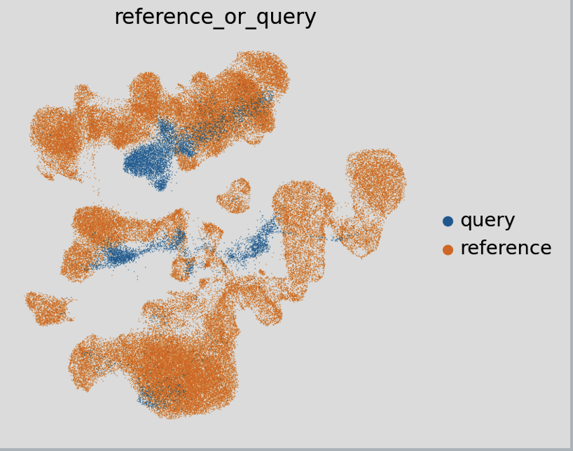
The overlap between the query and reference datasets is essential, as it forms the foundation for successful label transfer. scArches employs a k-nearest-neighbors approach to facilitate seamless and efficient label transfer. This method not only assigns labels but also generates valuable metrics that indicate the likelihood of the label assignments being accurate. Below, plots that illustrate this information are shown in detail.
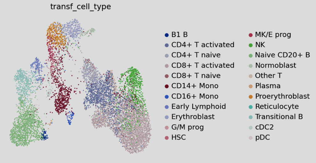
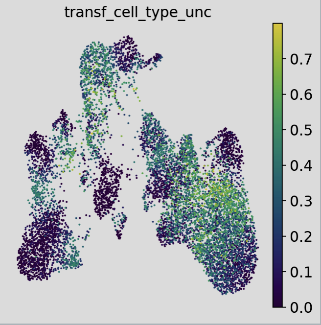
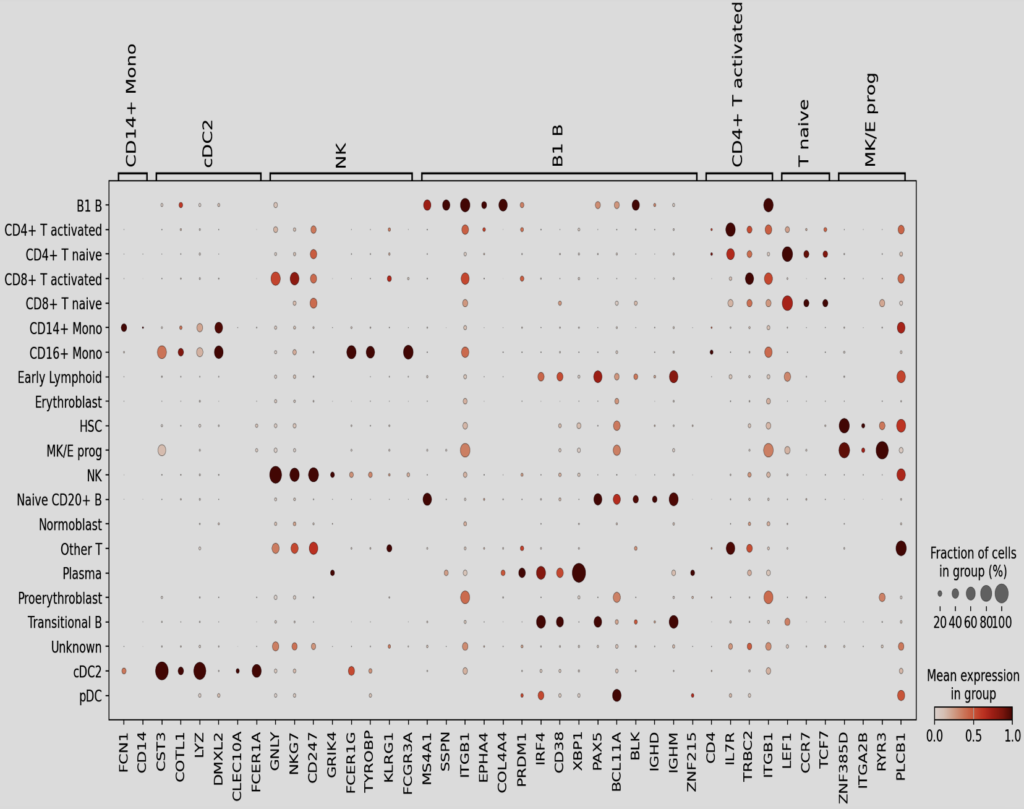
Interpreting these plots and determining appropriate cutoffs for label assignment is a nuanced process, often described as the “art” of annotation. Leveraging additional metadata from annotated objects can provide insights into cell types that may be misidentified. Prior expert knowledge of gene markers also plays a critical role in refining the annotations.
However, this process is far from perfected. The challenges highlight the importance of reference datasets, which have gained prominence as tools for standardizing annotations. Yet, as with any high-throughput technology, the quality of sample preparation is paramount. Technical variations introduced by individual operators or labs often become significant bottlenecks, hindering a universal and systematic label transfer process.
While batch effect correction algorithms, such as ComBat-seq, offer potential solutions to these issues, the ultimate resolution lies in alignment and standardization across laboratories sharing data. Lab automation and unified biological community standards represent the best long-term solutions—but these remain challenges for the future.
Conclusion
Once cell types are annotated in the single-cell RNAseq data, a range of analytical opportunities emerges to maximize the dataset’s value. Differential gene expression analysis can reveal genes uniquely expressed or regulated across cell types, potentially serving as markers for disease progression or therapeutic targets. Conducting gene set enrichment analysis within specific cell types could help identify dysregulated pathways and biological processes, shedding light on disease mechanisms. Assessing drug efficacy at the single-cell level provides insights into how various cell types respond to treatment, highlighting not only primary targets but also possible off-target effects and side effects of the drug. By integrating this data with pharmacogenomic databases, predictions of drug responses could become more refined. Additionally, trajectory and pseudotime analyses may help map developmental pathways and transitions between cell states, offering clues about stages of disease progression. Combining these approaches could deliver comprehensive insights, informing precision medicine strategies and supporting the development of targeted therapies.
